Genre_Lists <- list(
    c('Religious', 'Christian', 'Gospel', 'Religion', 'Catholic', 'worship'),
    c('Urban', 'R&B', 'Blues', 'Rhythmic','Rhythym and Blues','Hip Hop',
     'mainstream urban', 'Urban adult contemporary', 'Urban contemporary'),
    c('Pop', 'Contemporary Hit', 'adult contemporary', 'Top 40 (CHR)',
    'Hot AC', 'CHR'),
    c( 'Rock', 'Alternative','Indie'),
    c('Country','Southern', 'Bluegrass'),
c('News', 'News/Talk', 'Talk'))Exploring the Distribution of Radio Stations Across the U.S.
STA/ISS 313 - Project 1
Abstract
This project aims to examine trends in radio stations across the United States. It explores if there are regional trends in the genre of radio stations in each state and also studies the relationship between population density and the number of radio stations in each state. We used various plotting methods to analyze potential trends in our data. We concluded that there was not a strong trend in the data regarding the relationship between region and genre. In addition, there is potential that a higher population is correlated to the number of radio stations in a state, but our results were not extremely conclusive.
Introduction
This dataset contains information concerning radio stations in all 50 states of the United States. The data was mined from the “Lists of Radio Stations in the United States” Wikipedia page in 2022 and contains information such as the abbreviated name or call sign of the radio station (call_sign), the channel (frequency), the licensee (licensee), the city where the station is located (city), the kind of content of the radio station (format), and the state where the radio station is located (city). All of these variables are categorical variables, and we will use external data to further analyze trends in our data.
Question 1: Popular Station Genres Across the U.S.
Introduction
In this question, we aim to examine where in the United States there is the highest concentration of radio stations and if that varies by the genre of the station. We are interested in seeing if there are regional patterns for a specific genre of radio station (e.g. urban music, religious music, talk stations), specifically on the state level.
In order to answer this, we will need to use the format column (which specifies the kind of radio station) so we can visualize potential patterns across the country. In addition, the state column of will be important to calculate the number of radio stations in each state. We selected this question because we were curious about what patterns may exist in the most popular genres of radio in the U.S., and we thought there may be some relationship between the popularity of a certain genre of radio and the region of that station. Throughout our research, we also take a closer look at certain states such as Texas, California, and Florida, and examine trends more closely to better understand the breakdown of radio stations in diverse states.
Approach
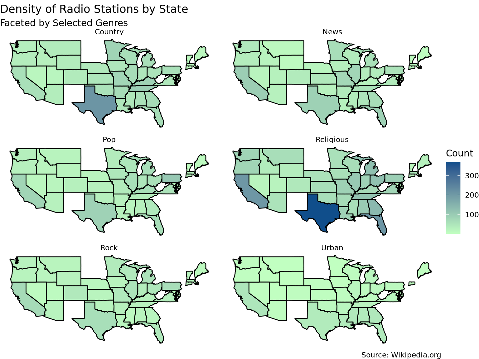
Our first plot will be a choropleth plot of the United States showing the number of radio stations present in each state, faceted by the genre. We selected this kind of density map because we thought it would make it easy to draw comparisons between states and visualize the patterns of where certain types of radio stations were the most prevalent. Prior to creating this plot, we had to bucket the various genres into broader categories. Initially, the format column had about 1,258 unique values. We decided to create 6 unique broad genres (chosen from the most popular radio station genres in Statista’s 2021 Global Consumer Survey ) and categorize the formats into those genres using a script. The first element of each list represents the name of that genre, and each list consists of keywords used to identify if one of the words from that list appeared in the format string, thus categorizing it as that genre.
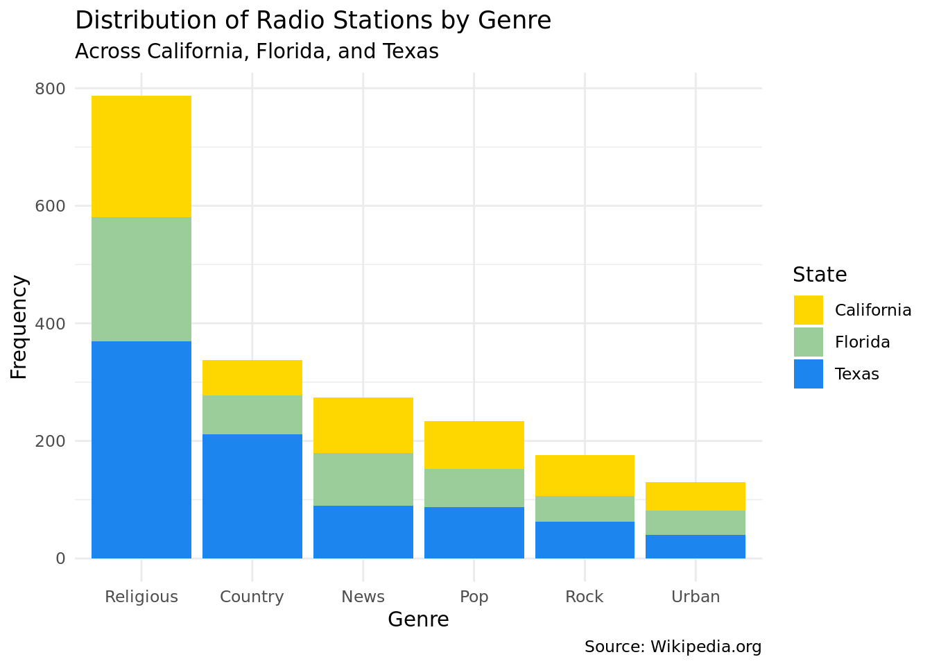
Our second plot is a bar chart that shows the number of radio stations from each genre across California, Texas, and Florida, three states that we determined from our choropleth map that had high concentrations of radio stations in a variety of genres. We figured a bar plot would be the best way to display the number of radio stations per genre in these three states, and coloring the states within the bars would enable effective comparison in the number of radio stations of that genre.
Analysis
Discussion
In the first plot, the trends are not very strong. News, Pop, Rock, and Urban all have a relatively consistent number of radio stations across the US. However, for the Country genre, Texas has a much higher concentration of radio stations than the rest of the states. In the Religion genre, Texas has by far the highest concentration with over 300 religious stations. Florida and California followed with somewhere around 200 stations in that category. Overall, we did not see very strong regional patterns for each genre of radio station. The spread of genres within the dataset was mostly even with the exception of the religion genre, which had the most observations. This is likely why the trends in the religion genre are more obvious; since there are more observations in this genre, the variation of density of stations across the US is easier to see.
For our second plot, we further our examination of the states with the most radio stations by focusing on the three that stuck out in plot 1 due to the overall higher density of radio stations compared to the other states: Texas, California, and Florida. The bar plot reveals that within these three states, the religion genre has by far the most stations at almost 800. Texas stations make up almost half of those stations. The genre with the second most stations across these states is country, which has a little over 300 observations. Again, Texas makes up the majority of these at about 200 stations within this category, the rest being fairly evenly split among California and Florida. The rest of the station genres across these states are News at a little under 300 stations, Pop at a bit over 200 stations, Rock with a little less than 200 stations, and lastly, Urban with a bit over 100 stations. Within these four genres, the spread of stations is rather even across the three states.
From these two plots, we can definitely conclude that Texas has overall more radio stations than most states, with the most popular genres being Religious and Country, which seems to make sense given the influence of the culture for a state in the South that is still predominantly influenced by the Christian religion. It is definitely important to consider the fact that we created these genres using key words from the original format column and there are some observations that were not included if their format did not fit well into one of our categories. Although we did review the radio stations in our new genres and which stations were, this certainly could have affected our visualization and interpretation of the results.
Question 2: Identifying correlation between population size and the number of radio stations in various states/regions of the United States
Introduction
Population size and density varies across the United States. For example, according to World Population Review (https://worldpopulationreview.com/state-rankings/state-densities), in 2023 Wyoming had a population of 581,075 and a population density of about 6 people per square mile. Meanwhile, New York has a population of 19,300,000 people and a population density of about 410 people per square mile. Given this radical variability in population and population density, it may be possible to find a correlation between these quantities and the variability in the number of radio stations in each state. Exploring this relationship may help us understand how a population or population density influences the number of radio stations that exist in a particular state or region. We will be using data from the state-stations dataset and the census population dataset. We will need the state, population and region variables along with a variable to represent the number of radio stations in a state for these visualizations.
Approach
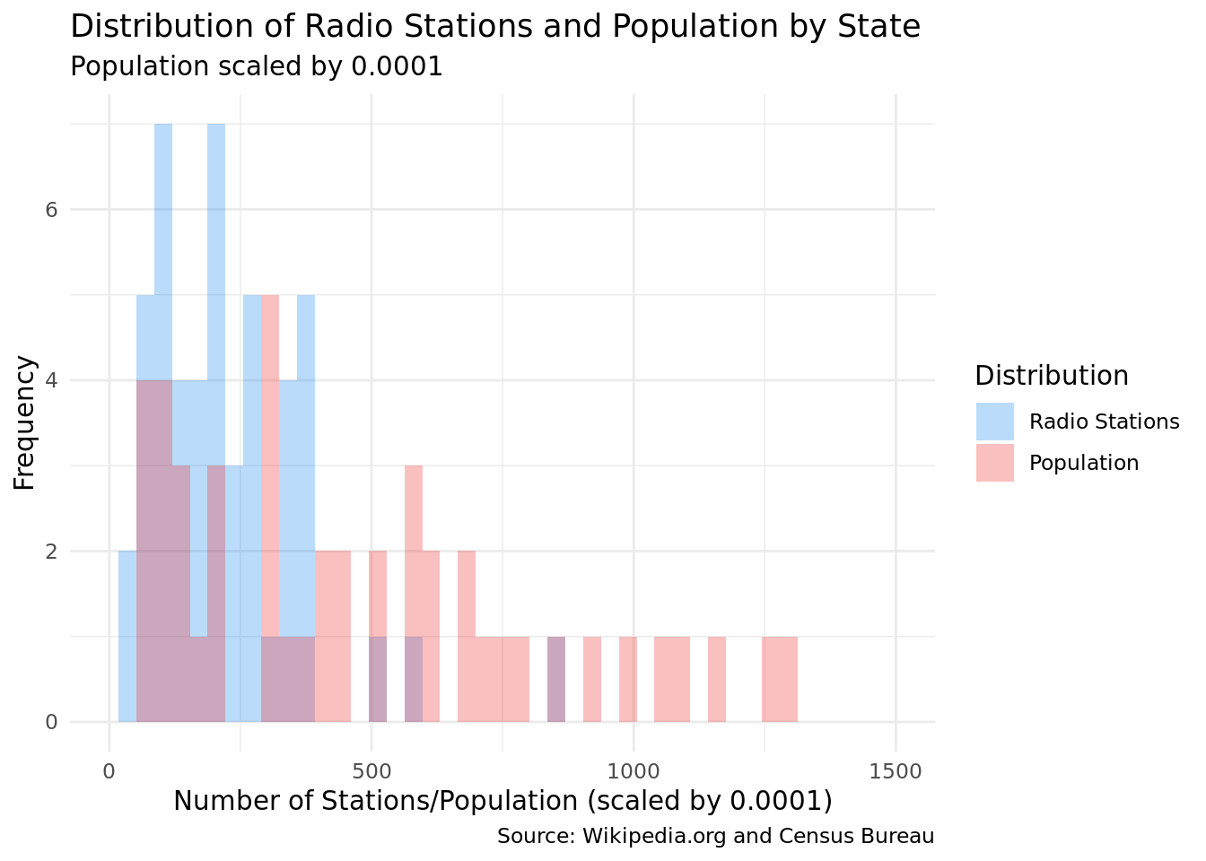
In the first plot we are going to investigate the relationship between the population and the number of radio stations by state. To address this question, we are going to layer the two distributions using a histogram plot where x-axis is the number of radio stations and the population size scaled by 0.0001. Histograms can help us easily see the frequency and overall distribution of each to identify interesting characteristics in the shape, spread, outliers, etc.
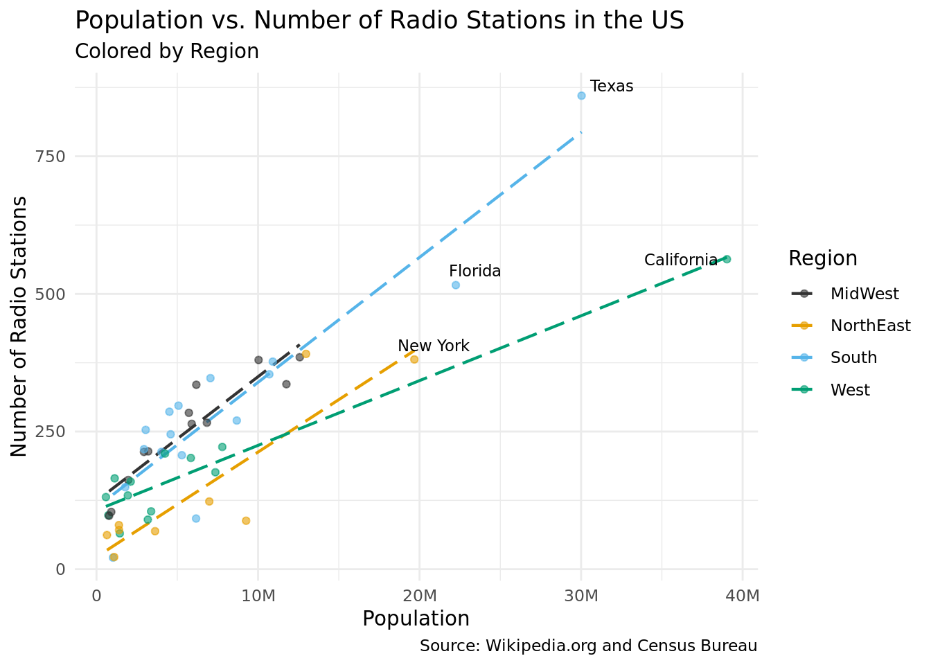
To further explore this relationship, we will need to create a scatterplot that plots each state as a point where the x-axis represents the population of a state and the y-axis represents the number of radio stations in the state. Each point will be color-coded to a particular region of the US based on the state. The scatter plot will be an effective visualization because it makes it easy to identify trends based on the distribution of all 50 data points. Identifying the region of points by color will help us search for unique trends in the relationship between population and radio stations based on region. We will be using a dataset where each row represents a radio station and we will only need the ‘state’ variable. We will also be pulling data from the dataset on population in the US by state, where we will need to utilize the ‘population’ state and region variables. Our approach will require use to mutate the data on the radio station dataset so that it only provides the ‘count’ (number of radio stations) and the state corresponding to that value. We will then join this dataset with the population dataset. We will also mutate the ‘region’ variable, where we will assign a region to a row based on the ‘state’. From here, we will use ggplot to render our visualization with a scatterplot, a linear regression for each region and text labels of outlier data points.
Analysis
Discussion
It is hard to identify a relation between the two variables because the distribution of the number of radio stations seems to be different to the distribution of population size in US states. Both distributions show a right skew (population more so than radio stations) and the population variable appears to have a wider spread. There is a concentration of states with a population size around 250 on the x-axis (scaled by 0.0001, so approximately 2,500,000). Similarly, there is also a concentration of states with around 250 radio stations, meaning that for the left area of the graph, the number of radio stations by state could possibly have a relationship with the population size. However, we see that as the population size increases, the number of radio stations per state does not necessarily increase in relation. The population histogram extends to around 1,300 (which when scaled back is 13,000,000). We removed outliers (such as Texas and California) that would have extended the distribution further. These are further explored in the second plot.
The scatter plot reveals a few interesting trends in the data. The first and most obvious trend we can spot is that there is a positive correlation between a state’s population and the number of radio stations in a state. This trend is consistent across all regions of the US. We speculate that his trend exists because states with higher populations may tend to have a higher demand for radio stations. Another interesting trend that we identified was that southern and midwestern states tend to have a higher number of radio stations than north-eastern states given a particular population. One potential explanation for this is that southern and midwestern states have a higher demand for specific types of radio stations. For example, Alabama, a very religious state, may have a higher demand for religious radio stations than New Hampshire, a less religious state. Another possibility is that southern and midwestern states have larger rural populations, which may require the use of more radio stations to reach the isolated populus.