Statsquatch: A Data Expedition into Bigfoot Sightings

STA/ISS 313 - Project 1

Abstract

The legendary cryptid Bigfoot (also commonly known as .Sasquatch, Yeti, or Yowie) has been a vibrant part of American lore for over a century.¹ The data used for this project was adapted by Timothy Renner from the Bigfoot Field Researchers Organization digital database, and it provides details on the thousands of sighting in the United States recorded over the years – with the first observation dating all the way back to 1869. Given the focus of data on geographic and atmospheric variables surrounding the sightings, our motivating questions revolve around uncovering the relationship between these variables and observations of Bigfoot. We first investigated the most common state and region for Bigfoot sightings, finding that sightings in the West region are consistently most common over time – specifically in the Pacific states. Next, we investigated the relationship between precipitation conditions on the day of Bigfoot sightings and the number of sightings and found a notably high number of sightings occurring during precipitation (a median of at least 92% precipitation probability). Through these questions, this project sufficiently analyzes and highlights trends in some of the geographic and weather conditions most commonly associated with Bigfoot sightings.

Introduction

The Tibbles chose the Bigfoot dataset from TidyTuesday because of our shared predilection for the supernatural and the desire to know more about one of the most iconic creatures in the North American imagination. The dataset, which first became available on Data World in 2017, was created by Timothy Renner. The data itself mainly originates from a digital database publicly available on the Bigfoot Field Researchers Organization (BFRO) website; however, information on weather was collected by Renner from the Dark Sky API. The dataset contains 5,021 rows, with each row representing a separate Bigfoot sighting, and 28 columns, with each column providing details on the sighting. The columns can generally be categorized as either lengthier verbal descriptions of the sighting observations or a combination of numerical and categorical variables that describe details regarding time, geographic, and weather conditions.

Given the focus of the variables on geography and weather conditions, The Tibbles decided to investigate two questions about the variables’ association with the number of Bigfoot sightings: one that focused on geographic conditions, and one that focused on weather conditions – though following preliminary investigation, we decided to focus on precipitation in particular. We anticipated that analysis of the results from our chosen variables could provide insight on physical and social factors that impact human sightings of Bigfoot, or perhaps could even provide insight on the nature of Bigfoot himself. To that end, we utilized the following variables in this project:

• state: state where the sighting occurred

• season: season during which the sighting occurred

• latitude: latitude of the sighting (degrees)

• longitude: longitude of the sighting (degrees)

• date: date of sighting (YYYY-MM-DD)

• precip_probability: probability of precipitation (%)

• precip_type: type of precipitation

Additionally, we used formal U.S. Census classifications (from a separate data set) to link states to aggregated regions/divisions.

Question 1: How does the geographic distribution of Bigfoot sightings change over time?

Introduction

Our first question investigates the geographic distribution of Bigfoot sightings and how this distribution has changed over time, using the latitude, longitude, and date variables to determine the precise location and decade the observation occurred. Analyzing the distribution of sightings and furthermore changes over times could provide insights on patterns of the public’s relationship with paranormal phenomena, as well as the impact of media and popular culture on these beliefs. Each region and each generation in turn has different social and cultural beliefs, formed by the overarching history of the area and the events of the decade. Understanding these changes in the geographic distribution of sightings over time could also shed new light on this elusive creature.

Approach

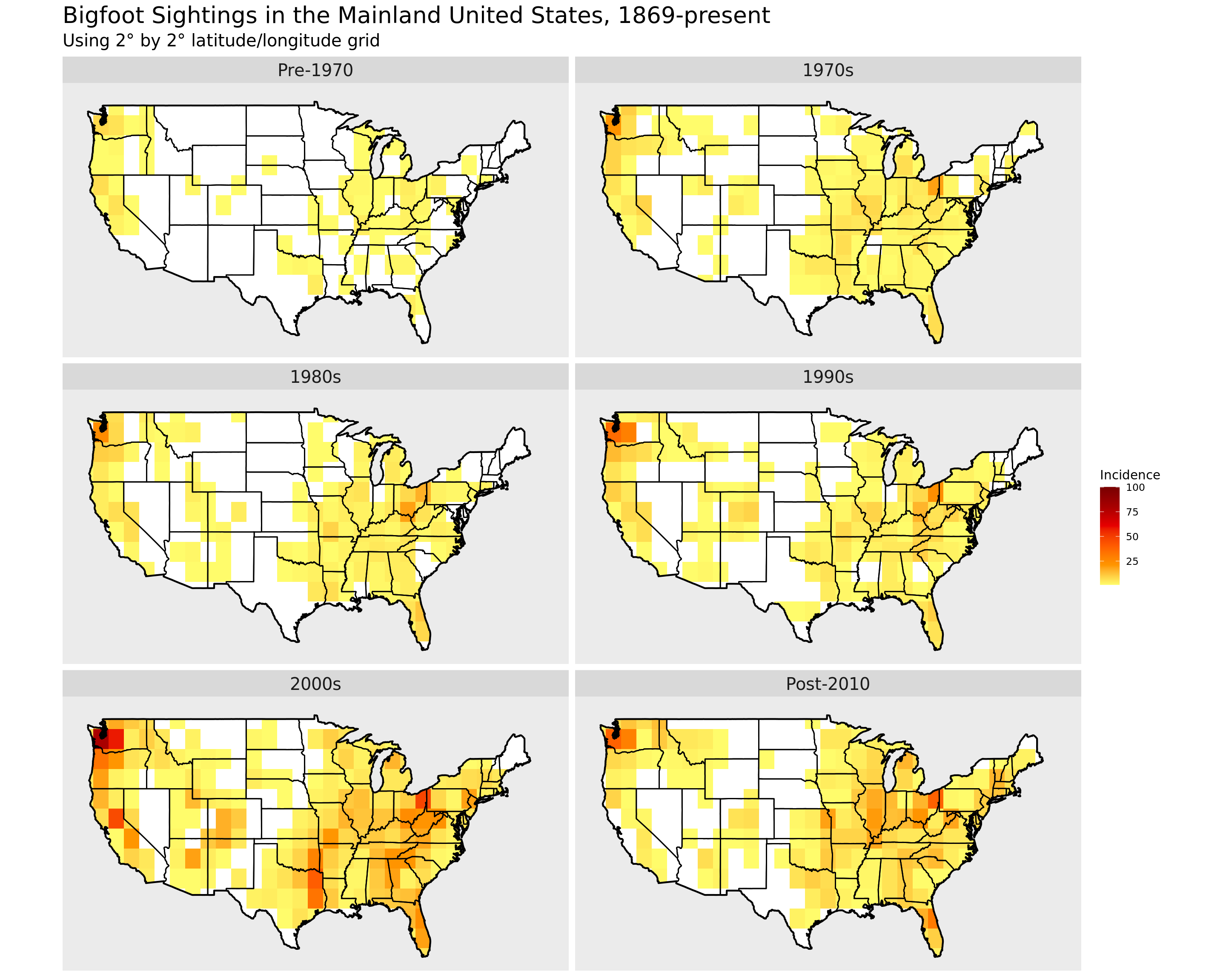
To address the first question, we utilized three different visualization techniques. The first method involved creating a scatter plot of Bigfoot sightings overlaid on a map of the mainland United States. This allowed us to visually observe clusters of sightings and areas of relative absence. The second method used a heat map of Bigfoot sightings overlayed on a map of the mainland United States. A heat map trades the precision of directly mapping all sightings for the advantage of a clear representation of density, which allowed for the identification of hot spots in regions with higher frequencies of Bigfoot sightings. We faceted both approaches by decade to facilitate comparisons across time.

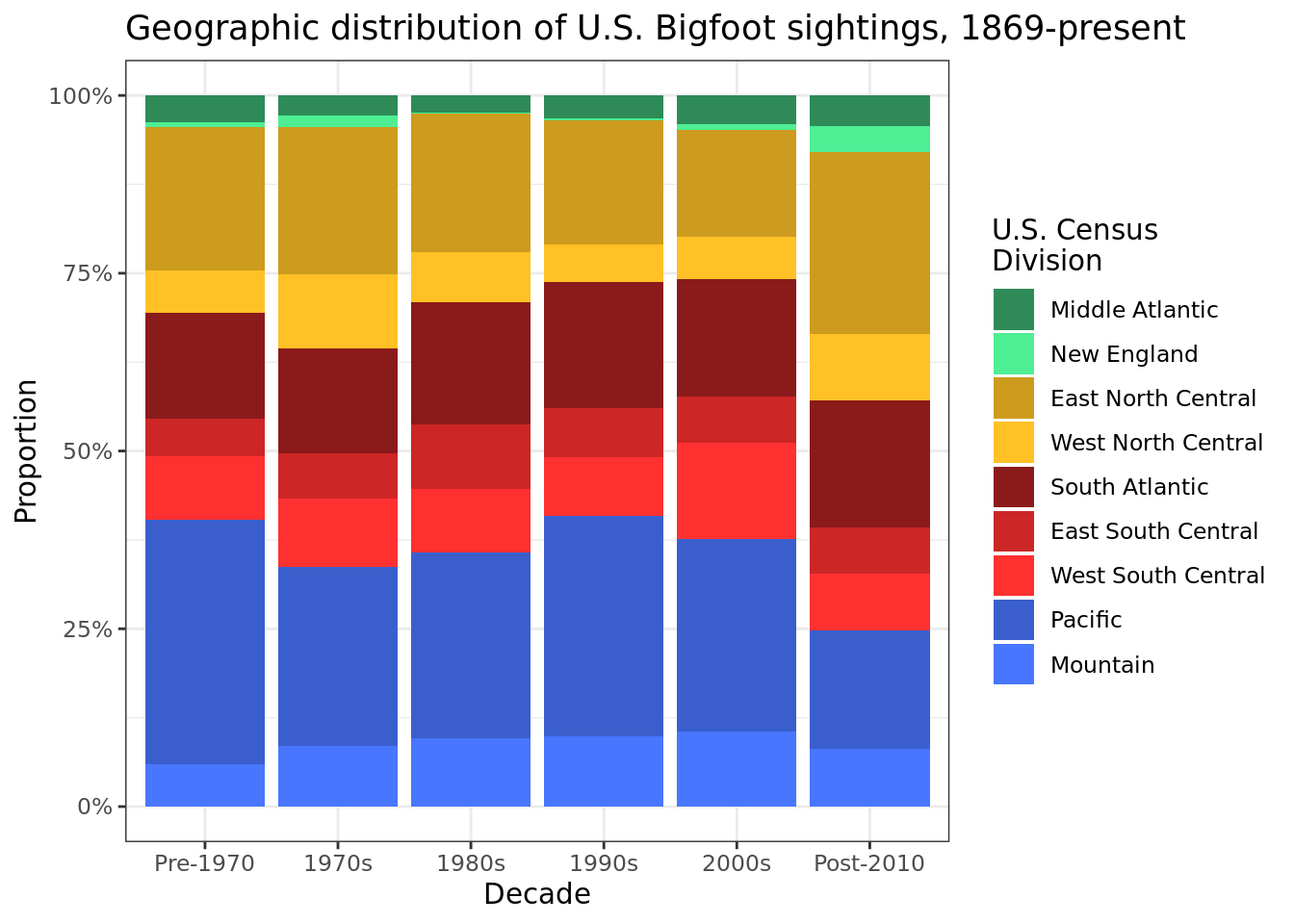
The third method employed a stacked bar graph to track the proportion of Bigfoot sightings recorded in each division of the country by decade. We used a stack bar graph to visualize changes in the distribution among divisions over time. While determining the exact proportion for a division was slightly more difficult in a stacked bar graph, the density of data was much greater than for a conventional bar plot that might display divisions in separate columns. We chose to graph proportions rather than nominal counts, as the focus of our research question was not the quantity of sightings, but rather the overall changes in the distribution as a whole. Additionally, some decades produced dramatically more sightings than others in the data set, making it difficult to observe trends in the less-populated decades of our data.

Analysis

Discussion

Our figures demonstrate that the geographic distribution of Bigfoot sightings has undergone significant changes over time. A few findings are clear nationwide— first, Bigfoot sightings have increased everywhere decade-over-decade. It is important to note, however, that earlier sightings may be less likely to appear in our data set. Beginning in the 2000s, Bigfoot was observed in areas where sightings had previously been absent, resulting in a wider geographic distribution, with sightings spanning the Dakotas, Plains States, and West Texas.

Another generalized finding— Bigfoot sightings ebb and flow in specific areas over time. To name just a few examples:

• During the 2000s, a range spanning from Eastern Texas to the Oklahoma/Arkansas border became a hot spot for Bigfoot sightings, despite having previously been a low-frequency area. The West South Central division, which includes Texas, Louisiana, Oklahoma, and Arkansas, doubled its proportion of national sightings from the 1990s to the 2000s, but this pattern dissipated after 2010.

• Even though its lush wilderness would be perfect Bigfoot real estate, New England saw very few Bigfoot sightings until the 1990s. This has changed— beginning in New York and moving eastward through Vermont, New Hampshire, all the way to Maine— Bigfoot has arrived, and this is visible in the heat-map. The New England census division was essentially barren of any sightings in the 1980s, but post-2010, it now contributes about 5% of the national total, outpacing its share of area.

• During the 2000s, Bigfoot sightings increased dramatically in the vicinity of Lake Tahoe and the Eldorado National Forest in California (identifiable both in the heat-map and scatter-plot). The grid-space containing this region actually set a record in the 2000s for the highest incidence outside of Washington State. Like the Texas hot spot, after 2010, this pattern completely disappeared. California is in the same region and division as Washington, limiting the conclusions we can draw from our bar plot that apply specifically to this pattern, but their (Pacific) division did see its proportion of sightings plummet post-2010, buttressing our conclusion from the heat-map.

Lastly, Bigfoot is moving east! After 2010, the median Bigfoot sighting jumped the Mississippi River into Illinois for the first time ever in our data. The heat-map explains why: downstate Illinois, northeast Ohio, and the Hudson River Valley have all become hot spots for Bigfoot sightings (the Ohio cluster actually dates all the way back to the 1970s). The West region of the U.S. — spanning from Honolulu to Denver— contributed 40% of the nation’s sightings in the 1990s, but this has fallen to only a quarter post-2010, actually disproportionately less than its area would warrant.

What this data, taken as a whole, tell us, is that the geographic distribution of sightings is highly variable. We venture two explanations: first, that Bigfoot’s tastes themselves are changing. Like all creatures, Bigfoot may have gotten bored and spread his wings- maybe for a yeti, Lake Tahoe was the place to be in 2007. Alternatively, we argue, Bigfoot sightings are a highly social event— people think they see Bigfoot and tell their family, friends, and even the media— making it much more likely that the individuals exposed to that information will earnestly (or for attention) claim to sight Bigfoot later. If one sighting can ‘trigger’ another, it would be logical for them to appear in geographical clusters like we observed forming and dissipating. While we cannot conclusively resolve the matter of Bigfoot’s existence, we hypothesize that the latter explanation is more likely.

Question 2: What precipitation conditions are most commonly associated with Bigfoot sightings?

Introduction

Our second question focuses on the relationship between precipitation and the frequency of Bigfoot sightings, examining the variables of precip_probability and precip_type. Through this analysis, we aim to uncover any associations between precipitation conditions and Bigfoot sightings. While legends surrounding precipitation weather events may overshadow those surrounding Bigfoot, these variables could potentially shed light on two aspects: first, they could help us better understand how physical weather factors influence human perception of the elusive creature; and second, they could lead to new hypotheses and discoveries about the nature of Bigfoot and its existence.

Approach

Note: Originally, we planned to examine the distribution of multiple weather variables, but ultimately decided to focus on precipitation due to its multiple variables (intensity, type, and probability) and potential relevance to Bigfoot sightings. After creating preliminary visualizations, we narrowed our analysis to precipitation type and probability, as the intensity values were heavily concentrated at or near 0.

To address our second question, we first created a box plot that displays the median probability of precipitation for each season. The precise meaning of precipitation probability is not well understood, but we assume it refers to the percentage of the forecasted area that is expected to receive precipitation. Given that meteorologists typically have quite a high level of precipitation prediction accuracy, The Tibbles assume that the probability value is more relevant to the percentage of area coverage. As all weather data in our dataset is aggregated by day and location, we first needed to establish the relationship between precipitation and the location of sightings to assess its relevance. The box plot is the best plot for this goal because it allows one to easily compare and evaluate the median probabilities for each season (labeled), while still providing important context about the range of probabilities that exist.

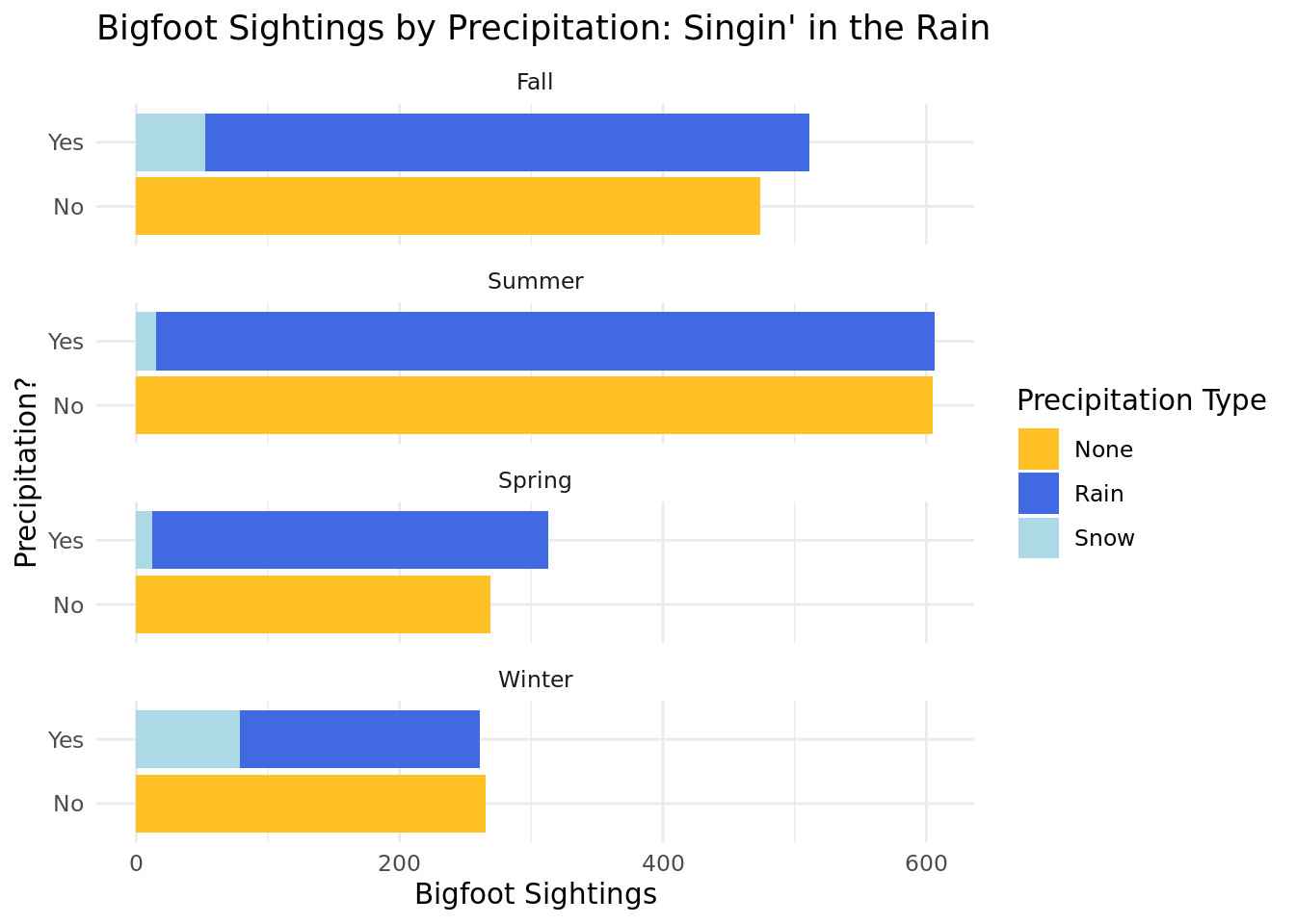
The second plot is a bar plot that compares the number of sightings in relation to precipitation and the type of precipitation (rain or snow), faceted by season. It is faceted by season to allow for the accounting of the profound impact that season can have on the presence and type of precipitation in our analysis. The bar plot allows for multiple easy comparisons, especially across facets: it allows for the comparison between number of sightings with and without precipitation, between precipitation within the presence of precipitation, and the previous two comparisons but between seasons. Given that in the United States, the majority of days throughout the year do not have precipitation, even a small difference between the number of sightings with and without precipitation can be telling. All these factors will be important in evaluating the existence and extent of an association between precipitation and a Bigfoot sighting.

Analysis

Discussion

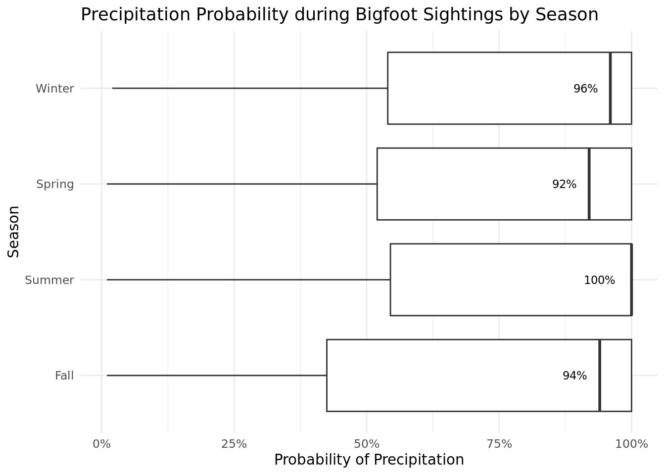
Our analysis revealed several interesting trends regarding the relationship between Bigfoot sightings and weather. The box plot indicated that there is a notably high probability of precipitation during Bigfoot sightings, with a median probability of 100% during the summer season. Even during the spring, the lowest probability of precipitation is still relatively high at 92%. One possible explanation for this finding is that Bigfoot might enjoy the rain or be more active during wet conditions. Alternatively, the high probability of rain could affect what people see, making it more difficult to differentiate between a Bigfoot and a tree or bush, for example.

The bar plot showed that the number of sightings on rainy days was almost equal to the number of sightings on sunny days, which was surprising given the disparity between the number of sunny and rainy days in the US. Additionally, there were more sightings during the summer season, which had more than twice the number of sightings than the winter or spring, and the fall season had almost twice as many sightings. This finding could be explained by the fact that more people are simply outside during the warmer months, leading to a higher chance of a sighting. Another possibility is that Bigfoot, like bears, hibernates during the colder months. This analysis sheds light on the possible influence of weather on Bigfoot sightings.

After an analysis of the visualizations, we find that the weather is a correlated with Bigfoot sightings, although we are unsure the direction of influence between the variables. The high probability of precipitation during Bigfoot sightings could indicate that Bigfoot is more active during wet conditions, or that the rain makes it more difficult for people to distinguish between Bigfoot and other objects. Given that there are more sunny days than rainy days in the United States, it is reasonable to consider that the weather may play a role in the frequency of Bigfoot sightings. The fact that the number of sightings on rainy days is almost equal to the number of sightings on sunny days does not necessarily mean that the weather is not a factor, but rather suggests that there are likely other factors at play as well. Therefore, it is possible that Bigfoot sightings are influenced by a combination of factors, such as weather, habitat, human activity, and other environmental factors. While our data does not provide a definitive explanation for the frequency of Bigfoot sightings, it does offer insights into potential patterns and trends. We encourgae further research into developing a deeper understanding of the relationship between Bigfoot sightings and weather conditions.

References

1. Magazine, S. (2018, September 1). Why do so many people still want to believe in Bigfoot? Smithsonian.com. Retrieved February 22, 2023, from https://www.smithsonianmag.com/history/why-so-many-people-still-believe-in-bigfoot-180970045/